Latent Growth Curve, Genome-Wide Association Study

Design the Model

Visit the Onyx website. Download Onyx, and create the pictured model.

LGC Model

In this model, we have four occasions of measurement for the phenotype (t1, t2, t3, and t4). There are two latent variables, int for the intercept and slope for the slope of the trajectory. The loadings from int to the manifests are all fixed to 1. In contrast, the loadings from slope to the manifests increase. In OpenMx, it is possible to use the actual date of measurement instead of time increments of 1 unit. However, the use of non-unit time increments would force us to estimate the model using maximum likelihood, a method much slower than weighted least squares. So we recommend unit time increments. The single nucleotide polymorphism (SNP) data will appear in the snp indicator. It will be convienent to use exactly the name snp because gwsem knows which column to use by its name.

We export the model. This model does not entirely suit our purpose. After copying the code to a file, we remove the bits relating to modelData. We will also need to make a few changes to accomodate covariates. To make these changes easier, we gather up all the mxPath statements into a list.

model export

library(gwsem)  # load gwsem

manifests<-c("t1","t2","t3","t4","snp")
latents<-c("int","slope")
path <- list(mxPath(from="int",to=c("t1","t2","t3","t4"), free=c(FALSE,FALSE,FALSE,FALSE), value=c(1.0,1.0,1.0,1.0) , arrows=1, label=c("int__t1","int__t2","int__t3","int__t4") ),
                 mxPath(from="slope",to=c("t1","t2","t3","t4"), free=c(FALSE,FALSE,FALSE,FALSE), value=c(0.0,1.0,2.0,3.0) , arrows=1, label=c("slope__t1","slope__t2","slope__t3","slope__t4") ),
                 mxPath(from="one",to=c("int","slope"), free=c(TRUE,TRUE), value=c(0.0,0.0) , arrows=1, label=c("const__int","const__slope") ),
                 mxPath(from="snp",to=c("slope","int"), free=c(TRUE,TRUE), value=c(1.0,0.0) , arrows=1, label=c("snp__slope","snp__int") ),
                 mxPath(from="int",to=c("int"), free=c(TRUE), value=c(1.0) , arrows=2, label=c("VAR_int") ),
                 mxPath(from="slope",to=c("slope","int"), free=c(TRUE,TRUE), value=c(1.0,0.1) , arrows=2, label=c("VAR_slope","COV_slope_int") ),
                 mxPath(from="t1",to=c("t1"), free=c(TRUE), value=c(1.0) , arrows=2, label=c("VAR_err") ),
                 mxPath(from="t2",to=c("t2"), free=c(TRUE), value=c(1.0) , arrows=2, label=c("VAR_err") ),
                 mxPath(from="t3",to=c("t3"), free=c(TRUE), value=c(1.0) , arrows=2, label=c("VAR_err") ),
                 mxPath(from="t4",to=c("t4"), free=c(TRUE), value=c(1.0) , arrows=2, label=c("VAR_err") ),
                 mxPath(from="snp",to=c("snp"), free=c(TRUE), value=c(1.0) , arrows=2, label=c("snp_res") ),
                 mxPath(from="one",to=c("t1","t2","t3","t4","snp"), free=F, value=0, arrows=1))
model <- mxModel("lgc", 
                 type="RAM",
                 manifestVars = manifests,
                 latentVars = latents,
                 path)

Simulate Fake Data

Even if we actually had real data, it might be useful to simulate fake data to develop expertise with our model and better understand what to expect from the real analyses. When we built the model in Onyx, we were careful to set starting values that were also appropriate for data simulation. Due to this preparation, data are easily simulated. We simulate N=500 people because this is the amount of fake SNP data available in the gwsem package (in the extdata subdirectory).

sim1 <- mxGenerateData(model, N)
head(sim1)
#>            t1          t2          t3           t4        snp
#> 1 -0.90030568 -2.76207727 -1.74302449  -1.51132454 -0.5517681
#> 2  0.38002682  0.64091402 -2.18280492  -4.05113240 -0.4435763
#> 3  0.81462836  3.05638042  3.94927189   8.22320913  1.4450938
#> 4  0.63561858 -0.09053616 -2.86289891  -6.38403645 -2.2150893
#> 5 -0.05880976 -3.48976930 -6.56627163 -11.22682944 -2.3963544
#> 6  0.34556391 -1.11458800 -0.06797686   0.04056822  0.1383600

A placeholder snp column needs to exist in the sim1 data.frame, and will be replaced with each SNP when we run the GWAS. We add some covariates too.

for (ii in 1:5) {
  sim1[[paste0('pc', ii)]] <- rnorm(N)
}

Model Customization

To add covariates, we need to rebuild the model. To make it easy to rebuild the model, we saved all the mxPath statements in the path list (above). All these paths can be implemented in the new model by including the path list in the model construction. We add mxFitFunctionWLS to select the weighted least squares fit function and add our simulated data.

m2 <- mxModel("lgc", type="RAM",
        manifestVars = model$manifestVars,
        latentVars = c(model$latentVars, paste0('pc', 1:5)),
        path,
        mxExpectationRAM(M="M"),
        mxFitFunctionWLS(allContinuousMethod="marginals"),
        mxData(observed=sim1, type="raw", minVariance=0.1, warnNPDacov=FALSE))

At this point, m2 almost corresponds with the output of buildOneItem or similar model building function. We just need to set up the covariates.

m2 <- setupExogenousCovariates(m2, paste0('pc', 1:5), paste0('t',1:4))

The model is ready to run. If we had ordinal indicators then we could use setupThresholds to perform some additional set up.

Running the GWAS

We run the model on the first SNP as a sanity check to ensure that our model is working correctly. The GWAS function writes parameter estimates to the given out.log file, but it also returns the model back to R. We can call summary on this model to see the results from the first SNP.

tdir <- tempdir()
dir <- system.file("extdata", package = "gwsem")
snp1 <- GWAS(m2, file.path(dir,"example.pgen"), file.path(tdir, "out.log"), SNP=1)
#> Running lgc with 29 parameters
#> Done. See '/tmp/RtmpA0vYb3/out.log' for results
summary(snp1)
#> Summary of lgc 
#>  
#> free parameters:
#>             name matrix   row   col      Estimate  Std.Error
#> 1       snp__int      A   int   snp  1.346320e-01 0.06260609
#> 2     snp__slope      A slope   snp -1.612135e-02 0.07187524
#> 3      pc1_to_t1      A    t1   pc1  6.345899e-02 0.06131007
#> 4      pc1_to_t2      A    t2   pc1  6.216955e-02 0.09368511
#> 5      pc1_to_t3      A    t3   pc1  1.266260e-01 0.13706537
#> 6      pc1_to_t4      A    t4   pc1  1.745729e-01 0.20093493
#> 7      pc2_to_t1      A    t1   pc2  1.400410e-02 0.06124550
#> 8      pc2_to_t2      A    t2   pc2 -1.663953e-01 0.08995065
#> 9      pc2_to_t3      A    t3   pc2 -2.321053e-01 0.14494158
#> 10     pc2_to_t4      A    t4   pc2 -4.847068e-01 0.20726968
#> 11     pc3_to_t1      A    t1   pc3  1.760877e-02 0.06315163
#> 12     pc3_to_t2      A    t2   pc3  5.117580e-02 0.10116807
#> 13     pc3_to_t3      A    t3   pc3  3.255096e-02 0.15652330
#> 14     pc3_to_t4      A    t4   pc3  5.058980e-02 0.23252581
#> 15     pc4_to_t1      A    t1   pc4 -8.962226e-02 0.06363051
#> 16     pc4_to_t2      A    t2   pc4 -7.390107e-02 0.09292618
#> 17     pc4_to_t3      A    t3   pc4 -8.978333e-03 0.15286037
#> 18     pc4_to_t4      A    t4   pc4  2.750599e-02 0.22062018
#> 19     pc5_to_t1      A    t1   pc5  7.404420e-02 0.06346138
#> 20     pc5_to_t2      A    t2   pc5  9.274255e-02 0.09248299
#> 21     pc5_to_t3      A    t3   pc5  9.359910e-02 0.14637978
#> 22     pc5_to_t4      A    t4   pc5 -1.022803e-01 0.20793700
#> 23       VAR_err      S    t1    t1  1.280021e+00 0.07604163
#> 24       snp_res      S   snp   snp  4.161738e-01 0.01347594
#> 25       VAR_int      S   int   int  8.238928e-01 0.12535132
#> 26 COV_slope_int      S   int slope -5.075074e-02 0.09848424
#> 27     VAR_slope      S slope slope  2.124818e+00 0.16100170
#> 28    const__int      M     1   int -7.436682e-05 0.05743234
#> 29  const__slope      M     1 slope -1.179730e-01 0.07014093
#> 
#> Model Statistics: 
#>                |  Parameters  |  Degrees of Freedom  |  Fit (r'Wr units)
#>        Model:             29                   2471             185.3371
#>    Saturated:             20                   2480               0.0000
#> Independence:             10                   2490                   NA
#> Number of observations/statistics: 500/2500
#> 
#> chi-square:  χ² ( df=16 ) = 185.3371,  p = 7.150818e-31
#> CFI: NA 
#> TLI: NA   (also known as NNFI) 
#> RMSEA:  0.1454893  [95% CI (0.1234642, 0.1682595)]
#> Prob(RMSEA <= 0.05): 1.110223e-16
#> To get additional fit indices, see help(mxRefModels)
#> timestamp: 2020-07-10 20:05:00 
#> Wall clock time: 0.425653 secs 
#> OpenMx version number: 2.17.4 
#> Need help?  See help(mxSummary)

This looks alright so we proceed to run all the SNPs and retrieve the results. The loadResults function calculates Z scores and P values for the snp__slope parameter. We might also examine the snp__int parameter.

GWAS(m2, file.path(dir,"example.pgen"), file.path(tdir, "out.log"))
#> Running lgc with 29 parameters
#> Done. See '/tmp/RtmpA0vYb3/out.log' for results
got <- loadResults(file.path(tdir, "out.log"), 'snp__slope')
got <- signif(got, 'snp__slope')

Some of the models failed to fit. If we’re interested to discover why then we can load these separately,

susp <- got[isSuspicious(got),]
head(susp)
#>    MxComputeLoop1 CHR    BP     SNP A1 A2 statusCode
#> 1:              7   1  8000  RSID_8  G  A       <NA>
#> 2:              9   1 10000 RSID_10  G  A       <NA>
#> 3:             16   1 17000 RSID_17  G  A       <NA>
#> 4:             18   1 19000 RSID_19  G  A       <NA>
#> 5:             20   1 21000 RSID_21  G  A       <NA>
#> 6:             23   1 24000 RSID_24  G  A       <NA>
#>                                                 catch1 snp__slope
#> 1: lgc.data: 'snp' has observed variance less than 0.1          1
#> 2: lgc.data: 'snp' has observed variance less than 0.1          1
#> 3: lgc.data: 'snp' has observed variance less than 0.1          1
#> 4: lgc.data: 'snp' has observed variance less than 0.1          1
#> 5: lgc.data: 'snp' has observed variance less than 0.1          1
#> 6: lgc.data: 'snp' has observed variance less than 0.1          1
#>    Vsnp__slope:snp__slope   Z   P
#> 1:                    NaN NaN NaN
#> 2:                    NaN NaN NaN
#> 3:                    NaN NaN NaN
#> 4:                    NaN NaN NaN
#> 5:                    NaN NaN NaN
#> 6:                    NaN NaN NaN

It looks like these SNPs had a variance below the threshold we specified in mxData (minVariance=0.1).

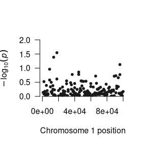
We can present a Manhattan plot consisting of the models that succeeded,

plot(got[!isSuspicious(got),])