Designing the Model
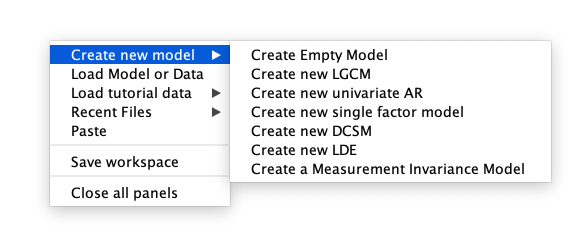
After opening the Onyx software, you will be greeted with a blank screen. To begin, right click on the screen and you will be prompted with a series of options. As we would like to create a new LGC model, choose Create new model > Create new LGCM.
First Step in Specifying the Onyx LGC Model
This will prompt you to set up some basic parameter of the latent growth model, such as the number of time points, where you would like to center the growth curve parameters, etc. In this example, we will use the following options:
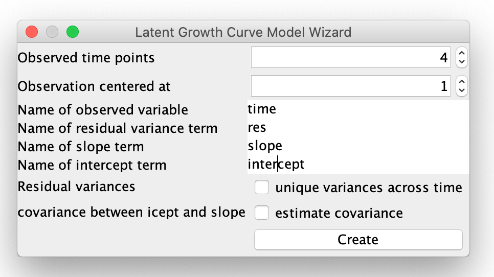
Specifying Options for the LGC Model
This will produce the following figure:
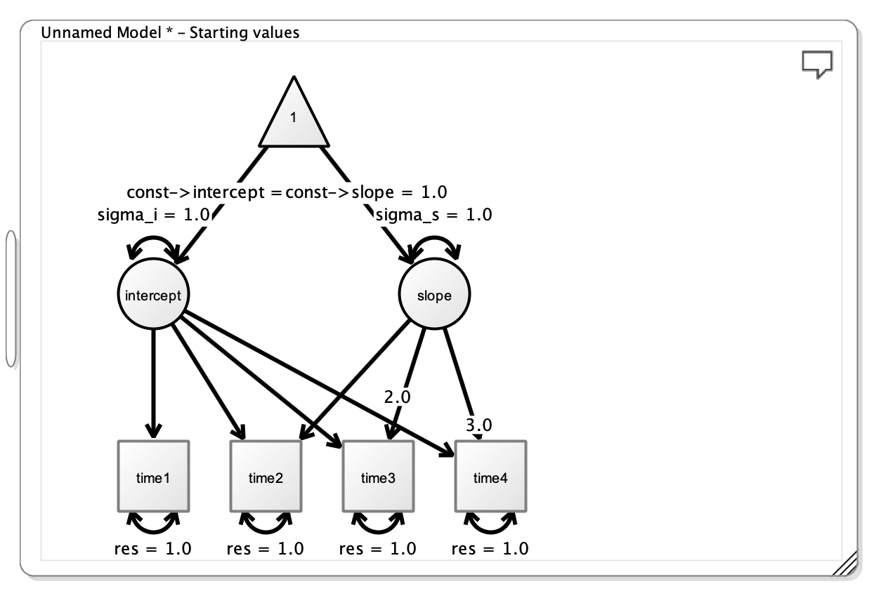
The initial Figure from Onyx
The next step is to add parameters to the model that we will need for the GWAS portion. Specifically, we will add 1) a name to the model, 2) the SNP, 3) regressions from the latent intercept and latent slope variables onto the SNP, and 4) a covariance between the intercept and the slope.
To name the model, right click on the canvas white space and several options will appear. In the text box, change the name to LCG GWAS.
To add the SNP, right click on the white space and click Create Variable > Observed. Then right click on the new box that appears and change the Variable name to SNP.
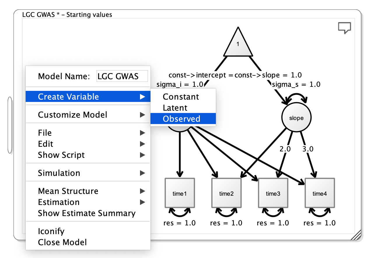
Adding the SNP to the Path Diagram
To add regressions paths from the SNP to the intercept and slope variables, right click on the new SNP variable and choose Add Path > Add Regression. You will want to do this for the intercept and the slope. Once the regression paths are in the diagram, right click on each and choose Free Parameter. This will tell the model to estimate values for these paths, which are the essential components for the GWAS.
To further customize the model, it is possible to estimate a covariance between the intercept and slope by right clicking on the intercept, choosing Add Path > Add Covariance, and then freeing the covariance path as was done for the SNP regressions.
Finally, we want to give the model sensible starting values, which can be done by right clicking on the respective paths and changing the value from the default 1.0 to a more sensible value. Better, but not perfect, starting values can increase the optimization speed.
Note that the loadings from the intercept to the manifests are all fixed to 1, and the loadings from slope to the manifests increase linearly, but are fixed at particular values (i.e. 0, 1, 2, 3). This is done as part of the LGC model.
At this point you have drawn a path diagram for a basic LGC GWAS model.
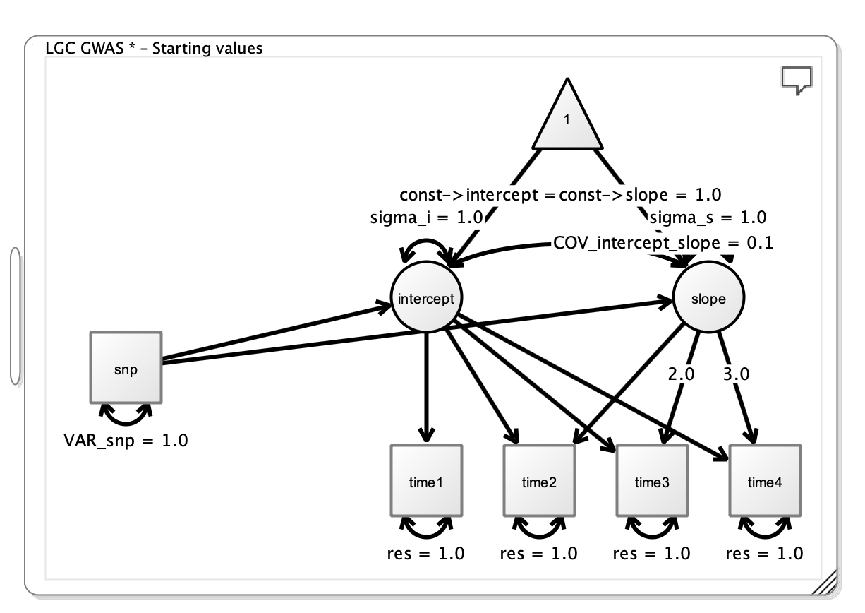
The Final Path Diagram from Onyx
Building the GWAS model in R
Once we have drawn the path model in Onyx, we can export the model syntax into a form that can be read by R, and customize it so that it can be read by GW-SEM. To export the model, right click on the white space and choose Show Script > OpenMx (Path). This will bring up a window at the top of the path diagram with syntax that can be copied into an R script.
It is now necessary to edit the code to remove irrelevant syntax and make a few changes to accommodate covariates. To make these changes easier, we gather up all the mxPath statements into a list.
This is the R Script that was generated by Onyx with the modifications highlighted.
location <- 'https://jpritikin.github.io/gwsem/gwsemCustomExample'

#
# This model specification was automatically generated by Onyx
#
library("OpenMx")                                                       # Edited
#> To take full advantage of multiple cores, use:
#>   mxOption(key='Number of Threads', value=parallel::detectCores()) #now
#>   Sys.setenv(OMP_NUM_THREADS=parallel::detectCores()) #before library(OpenMx)
modelData <- read.table(file.path(location, "lgcData.txt"), header = TRUE)                     # Cut
manifests<-c("time1","time2","time3","time4","snp")                      # Kept
latents<-c("intercept","slope")                                          # Kept
model <- mxModel("LGC_GWAS",                                             # Edited
type="RAM",                                                              # Cut
manifestVars = manifests,                                                # Cut
latentVars = latents,                                                    # Cut
mxPath(from="intercept",to=c("time1","time2","time3","time4"), free=c(FALSE,FALSE,FALSE,FALSE), value=c(1.0,1.0,1.0,1.0) , arrows=1, label=c("intercept__time1","intercept__time2","intercept__time3","intercept__time4") ),   # Edited
mxPath(from="slope",to=c("time2","time3","time4"), free=c(FALSE,FALSE,FALSE), value=c(1.0,2.0,3.0) , arrows=1, label=c("slope__time2","slope__time3","slope__time4") ),                                  # Edited
mxPath(from="one",to=c("intercept","slope"), free=c(TRUE,TRUE), value=c(1.0,1.0) , arrows=1, label=c("const__intercept","const__slope") ),                                             # Edited
mxPath(from="snp",to=c("intercept","slope"), free=c(TRUE,TRUE), value=c(0.5,0.1) , arrows=1, label=c("snp__intercept","snp__slope") ),                                                 # Edited
mxPath(from="intercept",to=c("intercept","slope"), free=c(TRUE,TRUE), value=c(1.0,0.1) , arrows=2, label=c("sigma_i","COV_intercept_slope") ),                                               # Edited
mxPath(from="slope",to=c("slope"), free=c(TRUE), value=c(1.0) , arrows=2, label=c("sigma_s") ),    # Edited
mxPath(from="time1",to=c("time1"), free=c(TRUE), value=c(1.0) , arrows=2, label=c("res") ),        # Edited
mxPath(from="time2",to=c("time2"), free=c(TRUE), value=c(1.0) , arrows=2, label=c("res") ),        # Edited
mxPath(from="time3",to=c("time3"), free=c(TRUE), value=c(1.0) , arrows=2, label=c("res") ),        # Edited
mxPath(from="time4",to=c("time4"), free=c(TRUE), value=c(1.0) , arrows=2, label=c("res") ),        # Edited
mxPath(from="snp",to=c("snp"), free=c(TRUE), value=c(1.0) , arrows=2, label=c("VAR_snp") ),        # Edited
mxPath(from="one",to=c("time1","time2","time3","time4","snp"), free=F, value=0, arrows=1),         # Edited
mxData(modelData, type = "raw")                     # Cut
);                                                  # Cut

result <- mxRun(model)                              # Cut
#> Running LGC_GWAS with 9 parameters
summary(result)                                     # Cut
#> Summary of LGC_GWAS
#>
#> free parameters:
#>                  name matrix       row       col    Estimate  Std.Error A
#> 1      snp__intercept      A intercept       snp -0.50984657 0.01754049
#> 2          snp__slope      A     slope       snp  0.09553418 0.01511185
#> 3                 res      S     time1     time1  1.00949655 0.01303252
#> 4             VAR_snp      S       snp       snp  0.98124812 0.01791512
#> 5             sigma_i      S intercept intercept  1.10473029 0.03430803
#> 6 COV_intercept_slope      S intercept     slope  0.05935154 0.02076271
#> 7             sigma_s      S     slope     slope  1.14262710 0.02468548 !
#> 8    const__intercept      M         1 intercept  1.89730586 0.01737536
#> 9        const__slope      M         1     slope  0.57037791 0.01496974
#>
#> Model Statistics:
#>                |  Parameters  |  Degrees of Freedom  |  Fit (-2lnL units)
#>        Model:              9                  29991              108303.5
#>    Saturated:             20                  29980                    NA
#> Independence:             10                  29990                    NA
#> Number of observations/statistics: 6000/30000
#>
#> Information Criteria:
#>       |  df Penalty  |  Parameters Penalty  |  Sample-Size Adjusted
#> AIC:       48321.49               108321.5                 108321.5
#> BIC:     -152603.66               108381.8                 108353.2
#> To get additional fit indices, see help(mxRefModels)
#> timestamp: 2020-07-10 20:23:04
#> Wall clock time: 0.5363045 secs
#> optimizer:  SLSQP
#> OpenMx version number: 2.17.4
#> Need help?  See help(mxSummary)
This is the edited R Script that we can modify for GW-SEM:
# This model that we will build on for GW-SEM

library(gwsem)
#>
#> Attaching package: 'gwsem'
#> The following object is masked from 'package:base':
#>
#>     signif

# load the LGC phenotypic data
lgcData <- read.table(file.path(location, "lgcData.txt"), header = TRUE)

# Use the Onyx Mode to edit the necessary components for the GWAS model
manifests<-c("time1","time2","time3","time4","snp")
latents<-c("intercept","slope")

path <- list(mxPath(from="intercept",to=c("time1","time2","time3","time4"), free=c(FALSE,FALSE,FALSE,FALSE), value=c(1.0,1.0,1.0,1.0) , arrows=1, label=c("intercept__time1","intercept__time2","intercept__time3","intercept__time4") ),
             mxPath(from="slope",to=c("time2","time3","time4"), free=c(FALSE,FALSE,FALSE), value=c(1.0,2.0,3.0) , arrows=1, label=c("slope__time2","slope__time3","slope__time4") ),
             mxPath(from="one",to=c("intercept","slope"), free=c(TRUE,TRUE), value=c(1.0,1.0) , arrows=1, label=c("const__intercept","const__slope") ),
             mxPath(from="snp",to=c("intercept","slope"), free=c(TRUE,TRUE), value=c(0.5,0.1) , arrows=1, label=c("snp__intercept","snp__slope") ),
             mxPath(from="intercept",to=c("intercept","slope"), free=c(TRUE,TRUE), value=c(1.0,0.1) , arrows=2, label=c("sigma_i","COV_intercept_slope") ),
             mxPath(from="slope",to=c("slope"), free=c(TRUE), value=c(1.0) , arrows=2, label=c("sigma_s") ),
             mxPath(from="time1",to=c("time1"), free=c(TRUE), value=c(1.0) , arrows=2, label=c("res") ),
             mxPath(from="time2",to=c("time2"), free=c(TRUE), value=c(1.0) , arrows=2, label=c("res") ),
             mxPath(from="time3",to=c("time3"), free=c(TRUE), value=c(1.0) , arrows=2, label=c("res") ),
             mxPath(from="time4",to=c("time4"), free=c(TRUE), value=c(1.0) , arrows=2, label=c("res") ),
             mxPath(from="snp",to=c("snp"), free=c(TRUE), value=c(1.0) , arrows=2, label=c("VAR_snp") ),
             mxPath(from="one",to=c("time1","time2","time3","time4","snp"), free=F, value=0, arrows=1))

# Package the components into a single GW-SEM Model

lgcGWAS <- mxModel("lgc", type="RAM",
        manifestVars = manifests,
        latentVars = c(latents, paste0('pc', 1:5)),
        path,
        mxExpectationRAM(M="M"),
        mxFitFunctionWLS(allContinuousMethod="marginals"),
        mxData(observed=lgcData, type="raw", minVariance=0.1, warnNPDacov=FALSE))

# Add the necessary covariates
lgcGWAS <- setupExogenousCovariates(lgcGWAS, paste0('pc', 1:5), paste0('time',1:4))

# Make sure that the model you specified runs properly and gives sensible parameter estimates
LGCtest <- mxRun(lgcGWAS)
#> Running lgc with 29 parameters
summary(LGCtest)
#> Summary of lgc
#>
#> free parameters:
#>                   name matrix       row       col      Estimate  Std.Error
#> 1       snp__intercept      A intercept       snp -0.4437830929 0.01830334
#> 2           snp__slope      A     slope       snp  0.1040938171 0.01530232
#> 3         pc1_to_time1      A     time1       pc1 -0.0133932530 0.01945328
#> 4         pc1_to_time2      A     time2       pc1 -0.0219015410 0.02431640
#> 5         pc1_to_time3      A     time3       pc1 -0.0347416791 0.03371482
#> 6         pc1_to_time4      A     time4       pc1 -0.0988534696 0.04570363
#> 7         pc2_to_time1      A     time1       pc2 -0.0039891552 0.01994979
#> 8         pc2_to_time2      A     time2       pc2  0.0166468586 0.02494595
#> 9         pc2_to_time3      A     time3       pc2 -0.0096845406 0.03450092
#> 10        pc2_to_time4      A     time4       pc2  0.0035911673 0.04674882
#> 11        pc3_to_time1      A     time1       pc3 -0.0257805372 0.01937684
#> 12        pc3_to_time2      A     time2       pc3 -0.0145290663 0.02410139
#> 13        pc3_to_time3      A     time3       pc3 -0.0343738802 0.03330934
#> 14        pc3_to_time4      A     time4       pc3 -0.0487441923 0.04556712
#> 15        pc4_to_time1      A     time1       pc4  0.0036696944 0.01978660
#> 16        pc4_to_time2      A     time2       pc4 -0.0005290562 0.02394867
#> 17        pc4_to_time3      A     time3       pc4 -0.0081206600 0.03343928
#> 18        pc4_to_time4      A     time4       pc4 -0.0234750570 0.04558151
#> 19        pc5_to_time1      A     time1       pc5 -0.0016405149 0.02020366
#> 20        pc5_to_time2      A     time2       pc5  0.0026169823 0.02486972
#> 21        pc5_to_time3      A     time3       pc5  0.0291196833 0.03433837
#> 22        pc5_to_time4      A     time4       pc5  0.0019723528 0.04608303
#> 23                 res      S     time1     time1  1.1190590789 0.01707673
#> 24             VAR_snp      S       snp       snp  0.9679213498 0.01796294
#> 25             sigma_i      S intercept intercept  1.1580268858 0.03650718
#> 26 COV_intercept_slope      S intercept     slope -0.0395421989 0.02189775
#> 27             sigma_s      S     slope     slope  1.1449532658 0.02594048
#> 28    const__intercept      M         1 intercept  1.8962909374 0.01737385
#> 29        const__slope      M         1     slope  0.5723508617 0.01498402
#>
#> Model Statistics:
#>                |  Parameters  |  Degrees of Freedom  |  Fit (r'Wr units)
#>        Model:             29                  29971             211.9503
#>    Saturated:             20                  29980               0.0000
#> Independence:             10                  29990                   NA
#> Number of observations/statistics: 6000/30000
#>
#> chi-square:  χ² ( df=16 ) = 211.9503,  p = 3.012665e-36
#> CFI: NA
#> TLI: NA   (also known as NNFI)
#> RMSEA:  0.04517908  [95% CI (0.03883452, 0.05172783)]
#> Prob(RMSEA <= 0.05): 0.9240899
#> To get additional fit indices, see help(mxRefModels)
#> timestamp: 2020-07-10 20:23:06
#> Wall clock time: 0.8249547 secs
#> optimizer:  SLSQP
#> OpenMx version number: 2.17.4
#> Need help?  See help(mxSummary)

library(curl)
curl_download(file.path(location, 'example.pgen'),
              file.path(tempdir(),'example.pgen'))
curl_download(file.path(location, 'example.pvar'),
              file.path(tempdir(),'example.pvar'))

# Run the GWAS Model
GWAS(lgcGWAS,
     file.path(tempdir(), "example.pgen"),
     file.path(tempdir(), "lgc.log"))
#> Running lgc with 29 parameters
#> Done. See '/tmp/RtmpnrCAuD/lgc.log' for results
The loadResults function calculates Z scores and P values for the snp__slope and snp__int parameters.
lr <- loadResults(file.path(tempdir(), 'lgc.log'), paste0('snp__', c('intercept','slope')))
LGCresInt <- signif(lr, 'snp__intercept')
LGCresSlo <- signif(lr, 'snp__slope')
In this example, we simulated snp1491 and snp1945 to be related to the latent intercept, and snp1339 and snp1598 to be related to the latent slope, and snp1901 to be related to both the intercept and the slope. We can look at the top SNPs using the head and order function to see whether the simulated SNPs are the most predictive of the latent variables.
head(LGCresInt[order(LGCresInt$Z, decreasing = T),])
#>    MxComputeLoop1 CHR   BP     SNP A1 A2 statusCode catch1 snp__intercept
#> 1:           1492   1 1491 snp1491  A  B         OK     NA     0.20668715
#> 2:           1946   1 1945 snp1945  B  A         OK     NA     0.18971924
#> 3:           1902   1 1901 snp1901  A  B         OK     NA     0.16039674
#> 4:           1625   1 1624 snp1624  A  B         OK     NA     0.10033048
#> 5:           1817   1 1816 snp1816  B  A         OK     NA     0.07273853
#> 6:            435   1  434  snp434  A  B         OK     NA     0.06541390
#>      snp__slope Vsnp__intercept:snp__intercept Vsnp__slope:snp__slope        Z
#> 1: -0.031280144                   0.0010574149           0.0006639955 6.356101
#> 2: -0.019634091                   0.0011138125           0.0007148516 5.684671
#> 3: -0.170852005                   0.0012745754           0.0007930931 4.492755
#> 4: -0.021632013                   0.0010447427           0.0006999388 3.104047
#> 5: -0.023473641                   0.0009348525           0.0006068575 2.378992
#> 6: -0.001020391                   0.0008092684           0.0005440612 2.299449
#>               P
#> 1: 2.069392e-10
#> 2: 1.310648e-08
#> 3: 7.030753e-06
#> 4: 1.908933e-03
#> 5: 1.736005e-02
#> 6: 2.147947e-02

head(LGCresSlo[order(abs(LGCresSlo$Z), decreasing = T),])
#>    MxComputeLoop1 CHR   BP     SNP A1 A2 statusCode catch1 snp__intercept
#> 1:           1902   1 1901 snp1901  A  B         OK     NA    0.160396742
#> 2:           1340   1 1339 snp1339  A  B         OK     NA    0.014354303
#> 3:           1599   1 1598 snp1598  A  B         OK     NA   -0.061215129
#> 4:           1627   1 1626 snp1626  A  B         OK     NA   -0.062642773
#> 5:            347   1  346  snp346  B  A         OK     NA   -0.005242869
#> 6:           1488   1 1487 snp1487  A  B         OK     NA   -0.013391246
#>     snp__slope Vsnp__intercept:snp__intercept Vsnp__slope:snp__slope         Z
#> 1: -0.17085200                   0.0012745754           0.0007930931 -6.066777
#> 2:  0.12980770                   0.0010761906           0.0007146684  4.855659
#> 3: -0.10829204                   0.0008830164           0.0005687600 -4.540796
#> 4:  0.03691133                   0.0009109517           0.0005948543  1.513402
#> 5:  0.03927281                   0.0011835840           0.0007568720  1.427515
#> 6:  0.03683034                   0.0010449434           0.0007029555  1.389127
#>               P
#> 1: 1.305030e-09
#> 2: 1.199870e-06
#> 3: 5.604224e-06
#> 4: 1.301775e-01
#> 5: 1.534314e-01
#> 6: 1.647942e-01
We can also present a Manhattan plot for the latent variable associations, or explore the data in other ways.