A schematic depiction of the Residuals Model
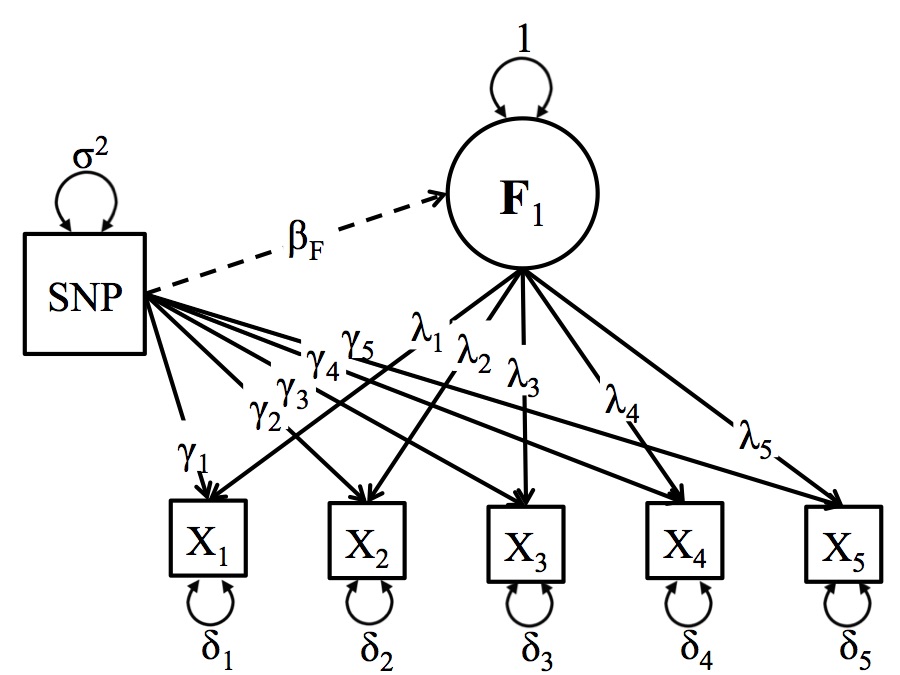
The Residuals GWAS Model is a variant of the One Factor GWAS Model where the SNP directly predicts one or more of the item-specific residuals, after accounting for the latent variable. The Figure below presents a schematic representation of the Residuals Model. The identification requirements are the same as for the one factor GW-SEM model. The notable difference is that the individual items are regressed on each SNP (γk). The residuals model allows researchers to regress a SNP on the residuals of the items that contribute to a latent factor. It is also possible to fit the residuals model so that the latent factor and a subset of the items are regressed on the SNPs. If you do this, in order to identify the SEM it is only possible to regress a subset of the items and the latent factor on the SNP or the model will not be identified.
In the Figure below, the circle (F1) is the latent factor, and the squares (xk) are observed indicators of the latent factor. The latent factor and observed indicators are connected by the factor loadings (λk). The residual variances (δk) represent the remaining variance in (xk) that is not shared with the latent factor. The regression of the observed items on the SNP (for all SNPs in the analysis) is depicted by (γk).
A schematic depiction of the Residuals Model
To demonstrate how to use the Residuals model function, we use the same simulated data that we used for the one factor GWAS model example. Specifically, we simulated data for 6,000 individuals consisting of 2,000 SNPs, three correlated items and 6 covariates (that are a proxy for age, sex, ancestry principle components or other confounds). The simulated data are loosely based upon the data used in the demonstration of Pritikin et al (under review). In the paper, we examined the association a latent substance use frequency variable that used tobacco, cannabis, and alcohol as indicators. The latent variable was regressed on each SNP with a minor allele frequency larger than 1%.
Note: Many of these steps are similar to those that you would take to run the One Factor GWAS.
The first step is opening R and loading the GW-SEM package into the R computing environment (which will also load all of the dependencies, such as OpenMx), which can be achieved by using the command below:
library(gwsem)
#> Loading required package: OpenMx
#> To take full advantage of multiple cores, use:
#>   mxOption(key='Number of Threads', value=parallel::detectCores()) #now
#>   Sys.setenv(OMP_NUM_THREADS=parallel::detectCores()) #before library(OpenMx)
#>
#> Attaching package: 'gwsem'
#> The following object is masked from 'package:base':
#>
#>     signif
The next step is to load the phenotypic data. This will include any items that define the latent variable or necessary covariates that you will include in the analysis, such as age, sex, or ancestry principle components. Once the phenotypic data has been loaded, it is advisable to make sure the data has been loaded properly. This can be done in a number of ways. For example, you can use the head command to inspect the first few lines of data, look at the means and variances, construct tables of ordinal variables, etc. If your data didn’t load properly, it will likely cause problems for the analysis and for the interpretation of the results.
location <- 'https://jpritikin.github.io/gwsem/gwsemOneFacExample'
phenoData <- read.table(file.path(location, "oneFacphenoData.txt"), header=TRUE)
head(phenoData)
#>       tobacco  cannabis    alcohol        pc1        pc2        pc3         pc4
#> 1  3.36379197 1.9456836  2.8611092  0.6581600 -0.1200383 -0.5039244  0.81789068
#> 2 -0.04339055 0.8374107  1.1329506 -0.4456708  1.6999452  0.2989812 -0.01336187
#> 3  2.34493591 1.7822021  1.2619447 -0.5075578  0.5317262  0.8304545 -1.08527994
#> 4  1.94136139 1.4179373  1.0871179 -0.2108447  0.9508879  0.1536526 -1.43699546
#> 5  1.07733966 0.9755835 -1.3167313  0.2835382 -1.6955112 -2.2021556  0.44969009
#> 6  1.63174525 1.0087218  0.7508155  0.4177546  0.3278404  0.2418577 -2.67388373
#>           pc5
#> 1  2.34856223
#> 2 -0.67114825
#> 3  0.02086144
#> 4  0.58885216
#> 5 -0.67308854
#> 6 -0.58135826
Once the data are loaded into R, you can recode the data, transform it, and tell R if we have ordinal or binary indicators using mxFactor(). The data for this example are simulated and continuous, and therefore, we will not be doing anything now, but if you would like to chop the indicators up into binary or ordinal variables, this would be when you would do it.
After you are satisfied that the data are in the appropriate shape we can build a one factor GWAS model with the following command:
                                                                                       # You must tell GW-SEM:
addFacRes <- buildOneFacRes(phenoData,                                                 # what the data object is (which you read in above)
                     itemNames = c("tobacco", "cannabis", "alcohol"),                  # what the items of the latent factor are
                     res = c("tobacco", "cannabis", "alcohol"),                        # the items you want to regress onto the SNP (the default is all of the items)
                     factor = F,                                                       # factor is set to F by default
                     covariates=c('pc1','pc2','pc3','pc4','pc5'),                      # what covariates that you want to include in the analysis
                     fitfun = "WLS")                                                   # and the fit function that you would like to use (WLS is much faster than ML)
Note about regressing the latent factor and SOME of the items on the SNPs: The model is not identified if both the latent variable and all of the items are simultaneously regressed on the SNP. In some cases, however, it may be important to understand the effect of the SNP on both the latent factor and the items. In such cases, you must remove at least path from the SNP to the item residuals, and then it is possible to toggle the factor argument from FALSE to TRUE.
You can take this object (addFacRes) which is technically an OpenMx model, and simply fit it using mxRun()
addFacResFit <- mxRun(addFacRes)
#> Running OneFacRes with 29 parameters
summary(addFacResFit)
#> Summary of OneFacRes
#>
#> free parameters:
#>               name matrix      row      col     Estimate  Std.Error lbound
#> 1   snp_to_tobacco      A  tobacco      snp  0.007166774 0.01831431
#> 2  snp_to_cannabis      A cannabis      snp  0.018824131 0.01849666
#> 3   snp_to_alcohol      A  alcohol      snp  0.035270907 0.01856413
#> 4   lambda_tobacco      A  tobacco        F  0.714703635 0.01407260
#> 5  lambda_cannabis      A cannabis        F  0.716511862 0.01378356
#> 6   lambda_alcohol      A  alcohol        F  0.712271688 0.01376622
#> 7   pc1_to_tobacco      A  tobacco      pc1  0.013600354 0.01324234
#> 8  pc1_to_cannabis      A cannabis      pc1  0.034214118 0.01342516
#> 9   pc1_to_alcohol      A  alcohol      pc1  0.006605336 0.01321714
#> 10  pc2_to_tobacco      A  tobacco      pc2  0.016604856 0.01294531
#> 11 pc2_to_cannabis      A cannabis      pc2 -0.012060134 0.01292010
#> 12  pc2_to_alcohol      A  alcohol      pc2 -0.014386349 0.01307769
#> 13  pc3_to_tobacco      A  tobacco      pc3  0.007312021 0.01300120
#> 14 pc3_to_cannabis      A cannabis      pc3  0.019124630 0.01285771
#> 15  pc3_to_alcohol      A  alcohol      pc3  0.019525141 0.01311066
#> 16  pc4_to_tobacco      A  tobacco      pc4 -0.024739970 0.01334323
#> 17 pc4_to_cannabis      A cannabis      pc4 -0.021984991 0.01300454
#> 18  pc4_to_alcohol      A  alcohol      pc4 -0.046430727 0.01291756
#> 19  pc5_to_tobacco      A  tobacco      pc5 -0.027658975 0.01294690
#> 20 pc5_to_cannabis      A cannabis      pc5  0.011439623 0.01315082
#> 21  pc5_to_alcohol      A  alcohol      pc5 -0.017530559 0.01315651
#> 22         snp_res      S      snp      snp  0.499413083 0.01288508  0.001
#> 23     tobacco_res      S  tobacco  tobacco  0.508562194 0.01505682  0.001
#> 24    cannabis_res      S cannabis cannabis  0.508357372 0.01474115  0.001
#> 25     alcohol_res      S  alcohol  alcohol  0.509128598 0.01438935  0.001
#> 26         snpMean      M        1      snp  1.020500000 0.00912717
#> 27     tobaccoMean      M        1  tobacco  0.712531627 0.02280868
#> 28    cannabisMean      M        1 cannabis  0.702877106 0.02296187
#> 29     alcoholMean      M        1  alcohol  0.685352413 0.02301247
#>    ubound
#> 1
#> 2
#> 3
#> 4
#> 5
#> 6
#> 7
#> 8
#> 9
#> 10
#> 11
#> 12
#> 13
#> 14
#> 15
#> 16
#> 17
#> 18
#> 19
#> 20
#> 21
#> 22
#> 23
#> 24
#> 25
#> 26
#> 27
#> 28
#> 29
#>
#> Model Statistics:
#>                |  Parameters  |  Degrees of Freedom  |  Fit (r'Wr units)
#>        Model:             29                  23971         7.011578e-17
#>    Saturated:             14                  23986         0.000000e+00
#> Independence:              8                  23992                   NA
#> Number of observations/statistics: 6000/24000
#>
#> chi-square:  χ² ( df=5 ) = 1.575792e-53,  p = 1
#> CFI: NA
#> TLI: NA   (also known as NNFI)
#> RMSEA: 0 *(Non-centrality parameter is negative)  [95% CI (0, 0)]
#> Prob(RMSEA <= 0.05): 1
#> To get additional fit indices, see help(mxRefModels)
#> timestamp: 2020-07-10 20:06:06
#> Wall clock time: 0.491261 secs
#> optimizer:  SLSQP
#> OpenMx version number: 2.17.4
#> Need help?  See help(mxSummary)
This is strongly advised, as it is a great time to test whether the model is being specified the way you want it to be and that you are not getting unexpected estimates.
Provided that the model looks reasonable, you can plug the model that you have built into the GWAS function using the command below:
library(curl)
curl_download(file.path(location, 'example.pgen'),
              file.path(tempdir(),'example.pgen'))
curl_download(file.path(location, 'example.pvar'),
              file.path(tempdir(),'example.pvar'))

GWAS(model = addFacRes,                                                                 # what model object you would like to fit
    snpData = file.path(tempdir(), 'example.pgen'),                                                        # that path to the snpData file.
    out=file.path(tempdir(), "FacRes.log"),                                                                # the file that you would like to save the full results into
    SNP=1:200)                                                                       # the index of the snps (how many) you would like to fit
#> Running OneFacRes with 29 parameters
#> Done. See '/tmp/Rtmp2Mjcyf/FacRes.log' for results
While the GWAS function will take a while and frequently be executed on a computing cluster, it is very useful to run a few SNPs (say 10 or 50) in an interactive session to ensure that: all of your relative file paths to the genotypes are correct, the model is taking a reasonable amount of time (i.e. 1-2 seconds/snp), the SNPs are giving sensible estimates, etc., as the results from a few SNPs can often tell you if there is a problem and that you are running a nonsensical model.
Refer to local documentation to learn how to submit jobs to your cluster queue submission systems. The R script that you provide will typically be similar to the one below:
library(gwsem)

phenoData <- read.table(file.path(location, "oneFacphenoData.txt"), header=TRUE)
head(phenoData)
#>       tobacco  cannabis    alcohol        pc1        pc2        pc3         pc4
#> 1  3.36379197 1.9456836  2.8611092  0.6581600 -0.1200383 -0.5039244  0.81789068
#> 2 -0.04339055 0.8374107  1.1329506 -0.4456708  1.6999452  0.2989812 -0.01336187
#> 3  2.34493591 1.7822021  1.2619447 -0.5075578  0.5317262  0.8304545 -1.08527994
#> 4  1.94136139 1.4179373  1.0871179 -0.2108447  0.9508879  0.1536526 -1.43699546
#> 5  1.07733966 0.9755835 -1.3167313  0.2835382 -1.6955112 -2.2021556  0.44969009
#> 6  1.63174525 1.0087218  0.7508155  0.4177546  0.3278404  0.2418577 -2.67388373
#>           pc5
#> 1  2.34856223
#> 2 -0.67114825
#> 3  0.02086144
#> 4  0.58885216
#> 5 -0.67308854
#> 6 -0.58135826

addFacRes <- buildOneFacRes(phenoData,                                                 # what the data object is (which you read in above)
                     c("tobacco", "cannabis", "alcohol"),                              # what the items of the latent factor are
                     covariates=c('pc1','pc2','pc3','pc4','pc5'),                      # what covariates that you want to include in the analysis
                     fitfun = "WLS")                                                   # and the fit function that you would like to use (WLS is much faster than ML)

GWAS(model = addFacRes,                                                                 # what model object you would like to fit
    snpData = file.path(tempdir(), 'example.pgen'),                                                        # that path to the snpData file.
    out=file.path(tempdir(), "facRes.log"))                                                                # the file that you would like to save the full results into
#> Running OneFacRes with 29 parameters
#> Done. See '/tmp/Rtmp2Mjcyf/facRes.log' for results
The next step is to read the results into R. The output from the GWAS function contains all of the estimates and standard errors for all parameters in the model (for each SNP), as well as other general model fitting information. While you are unlikely to want to read all of this output into R, it is useful to do this with a small test GWAS analysis to ensure that you are getting reasonable results and to familiarize yourself with what information is available, in case you need to explore a specific parameter or model in more detail. This can be done with,
More likely, you are going to want to focus on only the SNP regression coefficients. The loadResults function takes takes two arguments: the path to the data and the column name from the results file for the parameter that you want to examine.
Now that we have run the residual’s model, we have three parameters that we want to load into R. The function to do this is the same as for one parameter, but you need to do it three times. This obtains several R objects,
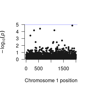
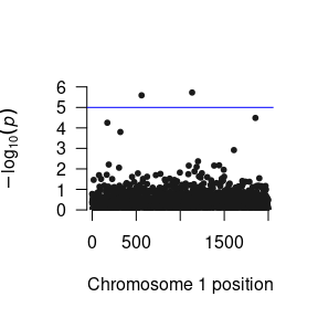
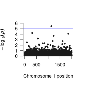
We can construct a Manhattan plot using the GW-SEM plot() function.
The loadResults() function formats the summary statistics from the analyses so that the data object can be seamlessly used by qqman, LDhub, and other post GWAS processing software.